The purpose of this project is to improve the reliability and accuracy of forecasting product demand for our firm. Historical estimates using total industry demand multiplied by our firm's market share have proven to be unreliable for use in allocating our firm's resources. Improving the formula we use to forecast demand will allow us to become more efficient.
Firm Demand (FD) = Total Industry Demand (TID) x Market Share (MS)
In the above equation:
Firm Demand (FD) = the quantity of Product produced by our firm which consumers can be expected to purchase in a period of time.
Total Industry Demand (TID) = the total quantity of Product which consumers can be expected to purchase in a period of time.
Market Share (MS) = the percentage of our firm's product which consumers can be expected to purchase in a period of time compared to the total quantity of all product purchased in the market during the same period of time.
Market share may also be expressed as:
Market Share (MS) = Relative Demand (RD) / Number of firms producing Product (N)
Where:
Relative Demand (RD) = the ratio of Firm Demand (FD) to the industry's average demand or Average Firm Demand (AFD)
Number of firms producing Product (N) = 10
Regression analysis will be performed on both TID and RD (response variables) to determine the effect predictor variables have on each. The predictor variables which we hypothesize might influence TID are time, average price in the market, and average advertising budget of all firms. The predictor variables, which we suspect will influence RD are the ratio of firm price to average market price, the ratio of firm advertising budget to average market advertising budget, and brand loyalty
Thus the Goal is clear. Predict TID and MS.
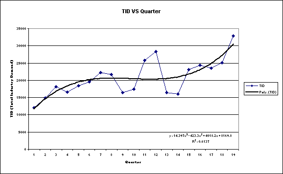
Figure
1: Graph and Trend Equation describing
Relationship between Quarter and TID
Above,
a polynomial trend curve on the order of 3 can be used to predict TID given the
Quarter. The R Square value is 0.6137,
which is a high correlation between the two variables.
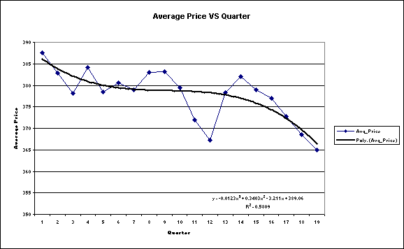
Figure
2: Graph and Trend Equation describing
Relationship between Quarter and Average Price
Above,
a polynomial trend curve on the order of 3 can be used to predict Average Price
given the Quarter. The R Square value
is 0.5809, which is a high correlation between the two variables.
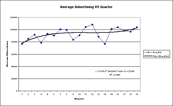
Figure
3: Graph and Trend Equation describing
Relationship between Quarter and Average Advertising
Above,
a polynomial trend curve on the order of 3 can be used to predict Average
Advertising given the Quarter. The R
Square value is 0.3499, which is a low correlation between the two variables.
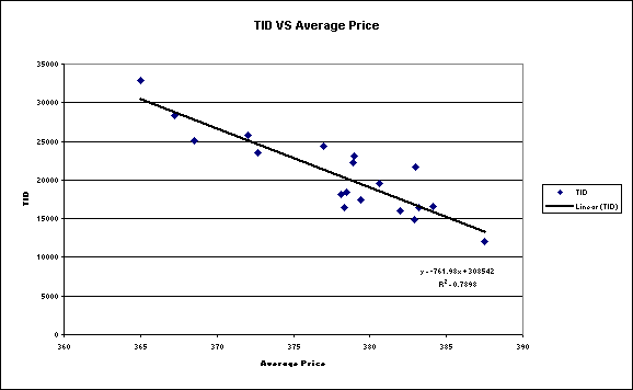
Figure
4: Graph and Trend Equation describing
Relationship between Average Price and TID
Above
a linear trend curve can be used to predict TID given the Average Price. An high R Square value of 0.7898 reveals a
high correlation between the two variables.
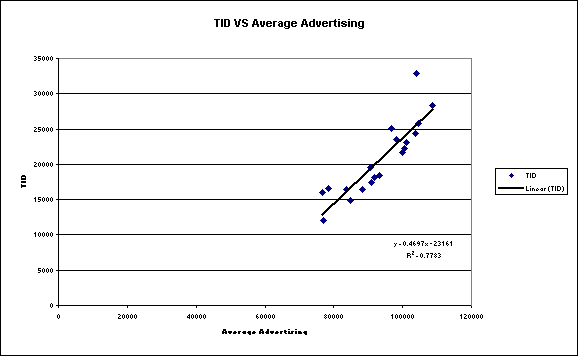
Figure
5: Graph and Trend Equation describing
Relationship between Average Advertising and TID
Above,
a linear trend curve can be used to predict TID given the Average
Advertising. An high R Square value of
0.7783 reveals a high correlation between the two variables.
|
|
Quarter |
Avg_Price |
Avg_Adv |
TID |
|
Quarter |
1 |
|
|
|
|
Avg_Price |
-0.703 |
1 |
|
|
|
Avg_Adv |
0.522361 |
-0.74883 |
1 |
|
|
TID |
0.694657 |
-0.88869 |
0.882219 |
1 |
Table
1: Correlation Matrix of TID, Average
Price, Average Advertising, and Quarter
From
the above matrix, Table 2 can be drawn, which rates the correlation of the
variable to each other with the most correlated being first.
|
Variables being Compared |
Rate |
Value of Correlation |
|
TID to Average Price |
1 |
0.88869 |
|
TID to Average Advertising |
2 |
0.882219 |
|
Average Advertising to
Average Price |
3 |
0.74883 |
|
Average Price to Quarter |
4 |
0.703 |
|
TID to Quarter |
5 |
0.694657 |
|
Average Advertising to
Quarter |
6 |
0.522361 |
Table 2: A table rating the correlation of each variable to one another
Table
2 shows that TID and Average Price are
most correlated, and Average
Advertising and Quarter are least correlated.
We
will now look at Relative Demand:
Relative Demand (RD) = the
firm’s demand as compared to the total industry demand.
RD = Firm Demand (FD) / Industry Average Demand (AFD)
Measures the firm’s demand as compared to industry demand, can indicate competitive edge
Industry Average Demand (AFD) = Total Industry
Demand (TID) / # Firms (N)
Relative Price (PREL) = Firm’s Price / Average
Industry Price
Relative price captures the firm’s pricing power as compared to the industry
Relative Advertising (AREL) = Firm’s Advertising Expenditures / Average Industry Advertising Expenditures
Relative advertising is a measure of firm
advertising expenditures as compared to the industry, can indicate whether a
firm is dependent on marketing for its product
Previous Quarter’s Relative
Demand (RD1) = Last Quarter’s Firm Demand / Last Quarter’s Total Industry
Demand. Previous Quarter’s Relative Demand is a measure of brand loyalty
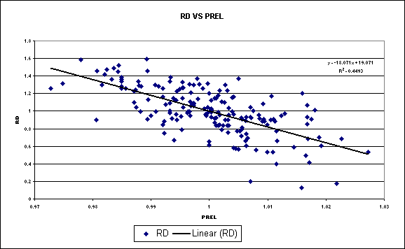
Figure
6: Graph and Trend Equation describing Relationship between PREL and RD
Figure
6 shows that there is a small relationship between PREL and the dependent
variable RD because using a linear trend line, the R Square value is
0.4493. This shows that the relative
price plays a role in affecting the relative demand.
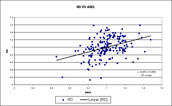
Figure
7: Graph and Trend Equation describing Relationship between AREL and RD
Figure
7 shows that there is a probably no relationship between AREL and the dependent
variable RD because using a linear trend line, the R Square value is
0.1431. This shows that relative
advertising insignificantly influences the relative demand.
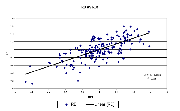
Figure
8: Graph and Trend Equation describing Relationship between RD1 and RD
Figure
8 shows that there is a good relationship between RD1 and the dependent
variable RD because using a linear trend line, the R Square value is
0.505. This shows that there is a
relationship between last quarter’s relative demand and the current quarter’s
relative demand.
|
Regression Statistics |
|
|
|
|
|
Multiple
R |
0.694657411 |
|
|
|
|
R
Square |
0.482548918 |
|
|
|
|
Adjusted
R Square |
0.45211062 |
|
|
|
|
Standard
Error |
3873.447436 |
|
|
|
|
Observations |
19 |
|
|
|
|
|
|
|
|
|
|
|
Coefficients |
Standard Error |
t Stat |
P-value |
|
Intercept |
14218.07018 |
1849.830412 |
7.686147922 |
6.26685E-07 |
|
Quarter |
645.9824561 |
162.2408597 |
3.981626191 |
0.000964868 |
Table
3: Regression analysis using Quarter to
estimate TID
Table
3 shows that since the P-value for both the intercept and Quarter are less than
0.05, then both of these coefficients are valid, but since the R Square is only
0.48, then there are other variables that more significantly affect TID.
|
Regression Statistics |
|
|
|
|
|
Multiple R |
0.952334882 |
|
|
|
|
R Square |
0.906941728 |
|
|
|
|
Adjusted R Square |
0.888330073 |
|
|
|
|
Standard Error |
1748.716231 |
|
|
|
|
Observations |
19 |
|
|
|
|
|
|
|
|
|
|
|
Coefficients |
Standard Error |
t Stat |
P-value |
|
Intercept |
130249.285 |
50620.06503 |
2.573076208 |
0.021204383 |
|
Quarter |
132.2282604 |
102.9946976 |
1.283835609 |
0.218677295 |
|
Avg_Price |
-358.6135195 |
122.1831725 |
-2.935048355 |
0.010239797 |
|
Avg_Adv |
0.263430426 |
0.063281565 |
4.162830481 |
0.000833208 |
Table 4: Regression analysis using Quarter, Average Price, and Average Advertising to estimate TID
Table
4 shows that since the P-value for Quarter is 0.21, which makes it safe to
assume that this coefficient is not applicable in calculating TID and it can be
thrown out. Average Price and Average
Advertising on the other hand do affect TID and another table must be computed
to accurately describe their relationship and R Square to TID.
|
Regression Statistics |
|
|
|
|
|
Multiple R |
0.946951041 |
|
|
|
|
R Square |
0.896716275 |
|
|
|
|
Adjusted R Square |
0.883805809 |
|
|
|
|
Standard Error |
1783.788804 |
|
|
|
|
Observations |
19 |
|
|
|
|
|
|
|
|
|
|
|
Coefficients |
Standard Error |
t Stat |
P-value |
|
Intercept |
164336.1704 |
43962.46954 |
3.738101434 |
0.001792219 |
|
Avg_Price |
-445.1684971 |
103.9426705 |
-4.282827208 |
0.000570731 |
|
Avg_Adv |
0.262728595 |
0.064548343 |
4.070260894 |
0.000890413 |
Table
5: Regression analysis using Average
Price and Average Advertising to estimate TID
Table
5 shows an applicable P-value and so the variables can be used in calculating
influence on TID. An R Square value of
0.90 shows a high correlation between both of these variables and their
influence on TID. This will be the
final model for TID. Equation 1
describes TID.
TID
= 164336.17 + (Average Price)*(-445.17) + (Average Advertising)*(0.26) (1)
|
Regression Statistics |
|
|
|
|
|
Multiple R |
0.978525574 |
|
|
|
|
R Square |
0.957512299 |
|
|
|
|
Adjusted R Square |
0.956783938 |
|
|
|
|
Standard Error |
0.056004573 |
|
|
|
|
Observations |
179 |
|
|
|
|
|
|
|
|
|
|
|
Coefficients |
Standard Error |
t Stat |
P-value |
|
Intercept |
16.12999601 |
0.444521299 |
36.28621627 |
2.37432E-83 |
|
RD1 |
0.533422048 |
0.016432467 |
32.46147126 |
5.6314E-76 |
|
Arel |
0.779630225 |
0.02694443 |
28.93474561 |
1.33291E-68 |
|
Prel |
-16.44445198 |
0.444138495 |
-37.02550482 |
1.0431E-84 |
Table
6: Regression analysis using RD1, AREL,
and PREL to estimate RD
Table
6 shows that since the P-value for all of the coefficients are acceptable, then
they are all valid in estimating RD.
The R Square of 0.96 is very high, thus showing that all of these
variable are applicable to determining the value of RD. This will be the final model for RD. Equation 2 describes RD.
RD
= 16.13 + (RD1)*(0.53) + (AREL)*(0.78) + (PREL)*(-16.44) (2)
Equation
3 is the model for calculating Firm Demand.
FD
= TID * MS = TID * (RD/N) (3)
Substituting
Equations 1 and 2 into Equation 3 and knowing that N = 10, yields Equation
4. Equation 4 is the final mathematical
model to estimate the demand for a product.
FD
= [164336.17 + (Average Price)*(-445.17) + (Average Advertising)*(0.26)]*[(
16.13 + (RD1)*(0.53) + (AREL)*(0.78) + (PREL)*(-16.44))/10] (4)
This formula is expressed in a table format
here: Table 7.